Home > finite state machines > Asyncronous FSM Design > Analysis of Asynchronous Sequential Machines
Analysis-of-Asynchronous-Sequential-Machines
Analysis of Asynchronous Sequential Machines :
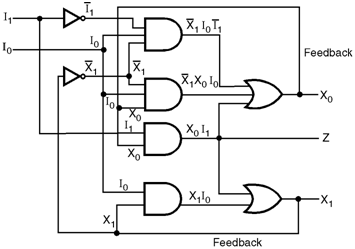
- Figure below shows a fundamental mode circuit. Note that flip flops are not being used.
- There are two feedback paths present in the circuit. X1 and X0 are the two state variables. These are applied to the gate inputs so as to generate the state variables.
- The feedback is essential in order to create the latching operations necessary to produce the sequential circuit.
- I0 and I1 are the two input variables and X0 and X1 are the state variables. Z is the output variable.
- The input state is dependent on the logic values of I0 and I1. The secondary state is dependent on the logic values of X0 and X1 whereas the total state depends on I0, I1, X0, and X1
Analysis of the Circuit :
- The next secondary states (denoted by X+0 and X+1 ) and the output Z are expressed as follows : X+1 = X0 I1 + X1 I0 …(2.5.1) X+0 = –X1 –I1 I0 + –X1 X0 I0+ X0 I1 …(2.5.2) Z = X0 I1 …(2.5.3)
- For the analysis of fundamental mode asynchronous sequential circuit, we need to create an input sequence.
- The total states are dependent on both the state variables as well as the input variables.
- For the fundamental mode, only one input variable should change its value of the given instant of time.
- We can construct a table which shows the present total state, next total state, whether the circuit is stable or unstable and the output variable Z.
- The present total state (X1, X0, I1, I0) is assumed and the corresponding next total state is obtained by using the next state from the next state secondary state equations
Present total state Next total state Stable total state Output
|
Present total state |
Next total state |
Stable total state |
Output |
||||||
|
X1 |
X0 |
I1 |
I0 |
X1 |
X0 |
I1 |
I0 |
Yes/No |
Z |
|
0 |
0 |
0 |
0 |
0 |
0 |
0 |
0 |
Yes |
0 |
|
0 |
0 |
0 |
1 |
0 |
1 |
0 |
1 |
No |
0 |
|
0 |
0 |
1 |
1 |
0 |
0 |
1 |
1 |
Yes |
0 |
|
0 |
0 |
1 |
0 |
0 |
0 |
1 |
0 |
Yes |
0 |
|
0 |
1 |
0 |
0 |
0 |
0 |
0 |
0 |
No |
0 |
|
0 |
1 |
0 |
1 |
0 |
1 |
0 |
1 |
Yes |
0 |
|
0 |
1 |
1 |
1 |
1 |
1 |
1 |
1 |
No |
1 |
|
0 |
1 |
1 |
0 |
1 |
1 |
1 |
0 |
No |
1 |
|
1 |
1 |
0 |
0 |
0 |
0 |
0 |
0 |
No |
0 |
|
1 |
1 |
0 |
1 |
1 |
0 |
0 |
1 |
No |
0 |
|
1 |
1 |
1 |
1 |
1 |
1 |
1 |
1 |
Yes |
1 |
|
1 |
1 |
1 |
0 |
1 |
1 |
1 |
0 |
Yes |
1 |
|
1 |
0 |
0 |
0 |
0 |
0 |
0 |
0 |
No |
0 |
|
1 |
0 |
0 |
1 |
1 |
0 |
0 |
1 |
Yes |
0 |
|
1 |
0 |
1 |
1 |
1 |
0 |
1 |
1 |
Yes |
0 |
|
1 |
0 |
1 |
0 |
0 |
0 |
1 |
0 |
No |
0 |
- When an input change (I1, I0) causes a secondary state change (X1, X0) and the next secondary state does not change, the total state is said to be stable. Transition Table :
- The information in Table can be rearranged into a transition table as shown in Figure below.
- Columns represent the input states (I1 I0 = 00, 01, 11, 10) and rows represent the secondary states (X1 X0 = 00, 01, 11, 10).
- The values of next secondary states (X+1 X+0 ) are written into the squares. Each entry in the square indicates a total state.
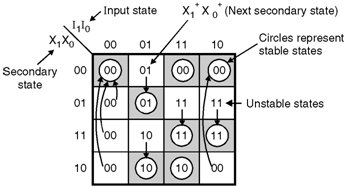
Transition table
- The circled secondary states in Figure are stable. The arrows indicate transitions from unstable states to stable states.